Showcases
The Julia language, combined with its powerful GPU ecosystem, enables developers and researchers to tackle demanding computational problems with unprecedented productivity and performance. With over 600 dependent packages, it is clear that Julia's GPU capabilities are not confined to a few niche areas; they are a foundational element empowering a vast and diverse scientific and engineering ecosystem:
Climate, Ocean, and Earth Sciences: Oceananigans.jl, GeophysicalFlows.jl, MagmaThermoKinematics.jl, PlanktonIndividuals.jl, RRTMGP.jl, SeisNoise.jl, vSmartMOM.jl
Physics & Engineering Simulation: MicroMagnetic.jl, Swalbe.jl, ParticleHolography.jl, MHDFlows.jl, Molly.jl, WaterLily.jl, Tortuosity.jl, Trixi.jl
Machine Learning & Artificial Intelligence: Flux.jl, Lux.jl, MeshGraphNets.jl, ObjectDetector.jl, LogicCircuits.jl
Quantum Science & Technology: Yao.jl, ITensor.jl, TensorOperations.jl
Biomedical & Medical Physics: KomaMRI.jl, NeuroAnalyzer.jl, Unfold.jl, Roentgen.jl
Bioinformatics & Computational Biology: Ebic.jl, SimSpread.jl
Numerical & Data Analysis: MonteCarloMeasurements.jl, Krylov.jl, MadNLP.jl, NextLA.jl, DistStat.jl, DifferentialEquations.jl
High-Performance Computing: ParallelStencil.jl, Dagger.jl
This diverse adoption underscores the power and flexibility of Julia's GPU tools. Now, let's dive into a few noteworthy examples in more detail:
Oceananigans.jl: Simulating Fluid Dynamics
Oceananigans.jl is a fast, friendly, and flexible Julia package for the numerical simulation of incompressible, stratified, rotating fluid flows on CPUs and GPUs. Developed as part of the Climate Modeling Alliance (CliMA), it's designed for both cutting-edge research into small-scale ocean physics and for educational purposes.
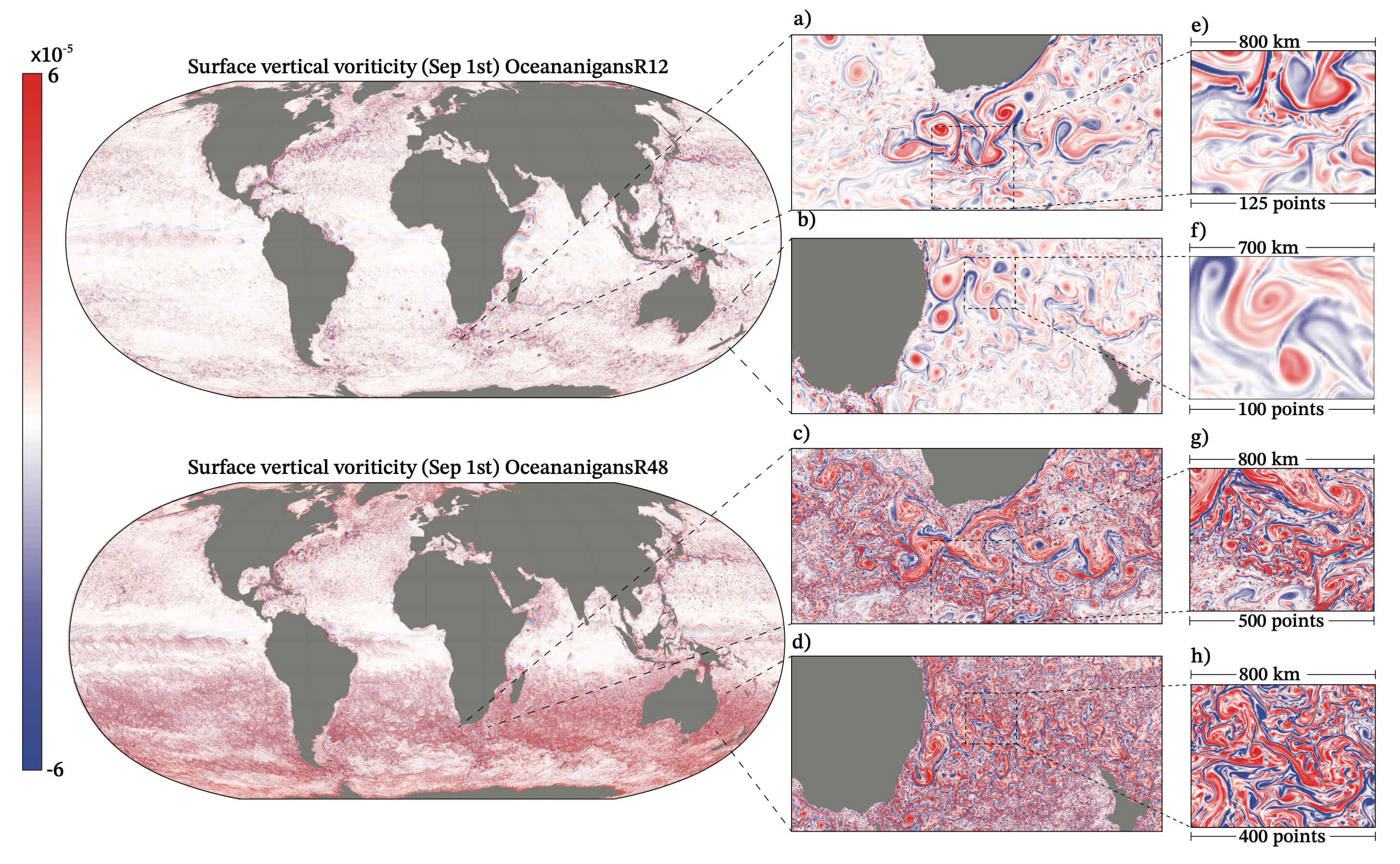
Vertical vorticity as simulated by Oceananigans after a one year integration.
Leveraging Julia and KernelAbstractions.jl, Oceananigans.jl achieves significant GPU speedups, often ~3x more cost-effective than CPU simulations and capable of handling ~150 million grid points on a single high-end GPU. These performance gains permit the long-time integration of realistic simulations, such as large eddy simulation of oceanic boundary layer turbulence over a seasonal cycle or the generation of training data for turbulence parameterizations in Earth system models
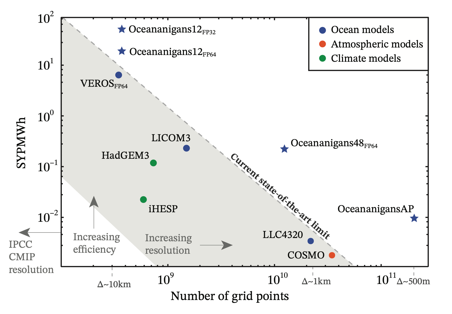
Simulated years computed by a megawatt-hour of energy (SWPMWh) versus
number of grid points for state-of-the-art atmosphere and ocean models.
GPU support in Oceananigans.jl is built on top of KernelAbstractions.jl, and simply requires the user to specify the GPU() backend when creating the grid:
using Oceananigans

grid = RectilinearGrid(GPU(), size=(128, 128), x=(0, 2π), y=(0, 2π),
                       topology=(Periodic, Periodic, Flat))
model = NonhydrostaticModel(; grid, advection=WENO())
ϵ(x, y) = 2rand() - 1
set!(model, u=ϵ, v=ϵ)
simulation = Simulation(model; Δt=0.01, stop_time=4)
run!(simulation)
DiffEqGPU.jl: Accelerating Scientific Simulation
Part of the acclaimed SciML ecosystem, DiffEqGPU.jl significantly accelerates the solution of large ensembles of differential equations (ODEs, SDEs). It provides highly optimized GPU kernels that enable substantial speedups for tasks like parameter sweeps, uncertainty quantification, and simulating complex systems in various scientific fields—often without requiring users to modify their existing model code.
DiffEqGPU.jl achieves high, vendor-agnostic performance. Benchmarks show it can outperform hand-optimized C++/CUDA solutions and run considerably faster (e.g., 20-100x) than vmap-based approaches in frameworks like JAX or PyTorch. This capability extends across NVIDIA, AMD, Intel, and Apple GPUs, largely due to its foundation on KernelAbstractions.jl.
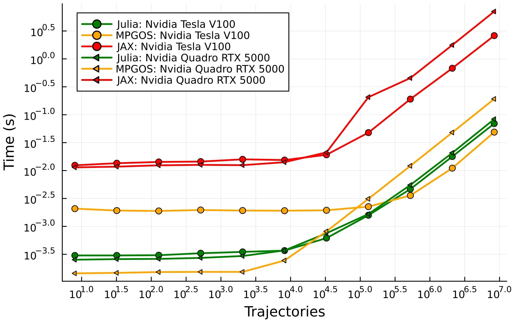
Solution time for an adaptive Lorenz ODE versus the number of trajectories.
The code changes required to solve this classical problem on the GPU are minimal. After setting up the ensemble of Lorenz equations, one can simply replace the EnsembleThreads() method with EnsembleGPUArray() to run the simulation on the GPU:
using DiffEqGPU, OrdinaryDiffEq, CUDA

function lorenz(du, u, p, t)
    du[1] = p[1] * (u[2] - u[1])
    du[2] = u[1] * (p[2] - u[3]) - u[2]
    du[3] = u[1] * u[2] - p[3] * u[3]
end

u0 = Float32[1.0; 0.0; 0.0]
tspan = (0.0f0, 100.0f0)
p = [10.0f0, 28.0f0, 8 / 3.0f0]
prob = ODEProblem(lorenz, u0, tspan, p)
prob_func = function (prob, i, repeat)
    remake(prob, p = rand(Float32, 3) .* p)
end
monteprob = EnsembleProblem(prob, prob_func = prob_func, safetycopy = false)

# CPU-based
sol = solve(monteprob, Tsit5(), EnsembleThreads(),
            trajectories = 10_000, saveat = 1.0f0);

# GPU-based
sol = solve(monteprob, Tsit5(), EnsembleGPUArray(CUDA.CUDABackend()),
            trajectories = 10_000, saveat = 1.0f0);
The use of EnsembleGPUArray has a bit of overhead because it parallelizes at the level of array operations. It is also possible to execute the entire solver on the GPU by using EnsembleGPUKernel, which offers even better performance, albeit at the the cost of some flexibility (such as using special solvers, and writing the problem in out-of-place form):
using DiffEqGPU, OrdinaryDiffEq, StaticArrays, CUDA

function lorenz2(u, p, t)
    σ = p[1]
    ρ = p[2]
    β = p[3]
    du1 = σ * (u[2] - u[1])
    du2 = u[1] * (ρ - u[3]) - u[2]
    du3 = u[1] * u[2] - β * u[3]
    return SVector{3}(du1, du2, du3)
end

u0 = @SVector [1.0f0; 0.0f0; 0.0f0]
tspan = (0.0f0, 10.0f0)
p = @SVector [10.0f0, 28.0f0, 8 / 3.0f0]
prob = ODEProblem{false}(lorenz2, u0, tspan, p)
prob_func = function (prob, i, repeat)
    remake(prob, p = (@SVector rand(Float32, 3)) .* p)
end
monteprob = EnsembleProblem(prob, prob_func = prob_func, safetycopy = false)

sol = solve(monteprob, GPUTsit5(), EnsembleGPUKernel(CUDA.CUDABackend()),
            trajectories = 10_000, saveat = 1.0f0)
Flux.jl: Elegant Machine Learning
Flux.jl is Julia's premier machine learning library, known for its 100% pure-Julia stack and lightweight abstractions. Flux is designed for flexibility, extensibility, and seamless integration with the broader Julia ecosystem. The package excels in allowing developers to easily express complex models, write custom layers or training loops, and leverage GPU acceleration with remarkable simplicity.
Here's an example of a simple multi-layer perceptron (MLP) model defined and trained on a synthetic dataset. The data is batched and subsequently moved to the GPU by using the device function, requiring minimal code changes:
using Flux
using CUDA # Or AMDGPU, Metal

# Function to move data and model to the GPU
device = gpu_device()

# Define our model, and upload it to the GPU
model = Chain(
    # multi-layer perceptron with one hidden layer of size 3
    Dense(2 => 3, tanh),
    BatchNorm(3),
    Dense(3 => 2)) |> device

# Generate some data on the CPU
noisy = rand(Float32, 2, 1000)
truth = [xor(col[1]>0.5, col[2]>0.5) for col in eachcol(noisy)]

# Training loop (processing the data in batches)
target = Flux.onehotbatch(truth, [true, false])
loader = Flux.DataLoader((noisy, target), batchsize=64, shuffle=true)
for epoch in 1:1_000
    for xy_cpu in loader
        # Upload the batch to the GPU
        x, y = xy_cpu |> device
        loss, grads = Flux.withgradient(model) do m
            y_hat = m(x)
            Flux.logitcrossentropy(y_hat, y)
        end
        Flux.update!(opt_state, model, grads[1])
    end
end